What Languages are Easy to Language-Model?

It’s been a while! I have been very busy with university for the past few months. Since I just ended the semester, I’d like to do these paper reviews more regularly. So stay tuned for more.

Today, we will be reading What Languages are Easy to Language-Model? A Perspective from Learning Probabilistic Regular Languages. I am currently working in multilingual language model in my internship, and I hope this paper will shed a light into the difference languages make in the development of LLMs… or at least that was my impression is before I read the paper.

After reading, I realize that this paper is mostly about finding a mathematical formalization of how well language models (LM) learn a certain distribution. Despite it being slightly different from what I expected, there is still a trove of interesting insights here.

Summary

This paper revolves around understanding the limits of LMs. Remember that LMs are just models that learn the representations of a certain token distributions. These distributions vary from languages to languages, and applications to applications. For example, a protein language model would have different distribution as compared to an English literary language model, obviously. However, despite the advancement of LMs, there is no formal guarantee on which distribution they can or cannot represent. This paper aims to provide that guarantee, or at least determine which distribution is easier to represent than others.

The authors extensively used Deterministic Probabilistic Finite-State Automata (DPFSA) to simulate language models, and then proved that any neural LMs that exactly matches DPFSA of rank $R$ must have hidden-state dimension $D$, where $D \geq R$ (Theorem 3.1). Any lower than $R$, the neural LMs won’t be able to represent the distribution properly.

Empirically, the authors generate random DPFSA of controller size and rank, then train RNN and Transformers on the sampled string, and measure their performance by calculating the KL-divergence to the true DPFSA distribution.

Neural LMs vs PFSAs

Before we dive into DPFSAs, let’s recall the two ends of the language modeling spectrum:

There has been a long-standing softmax bottleneck concern where low-rank $\mathbb{E}$ is unable to express all possible conditional distributions. To validate this, we need to compare with an automata with well-defined distribution, such as DPFSAs.

DPFSAs

A DPFSA is a PFSA with at most 1 outgoing transition for each state-symbol pair. More precisely:

• You have an alphabet $\Sigma$ and finite set of states $Q$.
• From each $q \in Q$ and $a \in \Sigma$, at most one transition $q\xrightarrow{\text{a/p}}q'$ exists, where $p$ is the transition probability.
• This results in determinism where each input string $y$ follows exactly one path through the automaton, resulting in a unique probability value.

Furthermore, a minimal DPFSA has no redundant and unreachable state. So each of its $Q$ states are used.

Using DPFSAs as Softmax-Layer LM

To bridge DPFSA and neural LMs, we observe that the DPFSA’s next symbol distribution can be written exactly as:

This is equation(3) in the paper, where:

• $h_A(y_{<t}) \in \{0,1\}^{|Q|}$ is the one-hot state of the automaton after seeing prefix $y_{<t}$.
• $T \in \mathbb{R}^{|\Sigma| \times |Q|}$ collects all transition and EOS logits. Note that this output matrix $T$ has the full-rank $|Q|$, but further in the paper, we often do not use the full rank, and refer $\text{Rank}(T) = R$.

Combining Everything

With this formulation in hand, we can determine that a minimal DPFSA one-hot vector spans the entire $\mathbb{R}^{|Q|}$. But multiplying by a rank $R$ matrix can only hit an $R$ dimensional subspace. Therefore, we get our very important core theory:

Theorem 3.1 (rephrased)
If a minimal DPFSA has rank $R$ then any representation-based neural LM that exactly matches its distribution must use at least $R$ dimensions in its final representation.

The best thing is that this theorem is architecture-agnostic. It holds for RNNs, LSTMs, Transformers, etc, as long as it ends in a linear + softmax layer.

Empirical Validation

To validate this theorem, the authors generate DPFSAs with controlled $|Q|, |\Sigma|$ and rank $R$ by sampling a Gaussian matrix. Each automaton serves as “text generator” generating some thousands of sample strings. Then they trained RNNs and Transformers of various hidden sizes $D$ on those samples and measure the KL-divergence $D_{KL}(p || q)$, where $p$ is DPFSA distribution and $q$ is neural LMs.

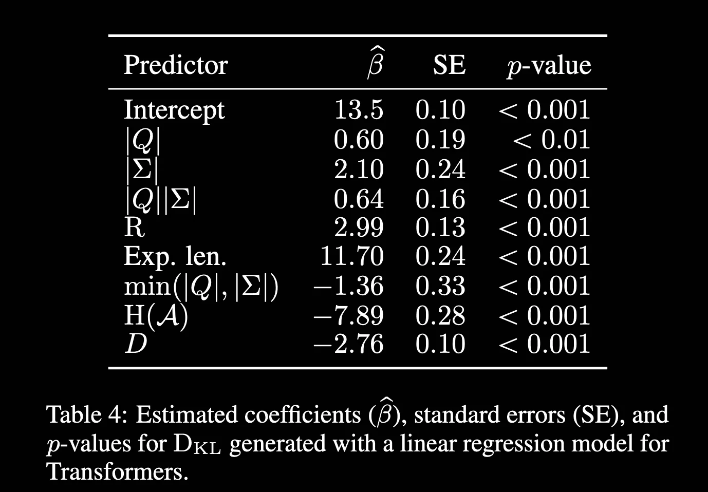
Here are the key findings (Table 4 in the paper):

1. As soon as $D < R$, KL-divergence spikes, confirming that $R$ is indeed the lower bound.
2. More states $|Q|$, symbols $|\Sigma|$ or expected length will widen the KL-divergence gap, but rank $R$ is the most dominant factor.
3. Most interestingly, automata with higher randomness (entropy) are easier to approximate by neural LMs.

The authors then did comparisons between RNNs and Transformers, where they found that RNNs generally found better distribution, showing the capabilities of RNNs in modeling formal languages right off the bat, while transformers still need careful language-specific hyperparameter tuning. The predictors in Table 4 also have different significance between transformers and RNNs. For example, $|Q|, |\Sigma|$ are strong predictors of transformers, but not RNNs.

Final Words

This paper delivered a clean, architecture-agnostic lower bound on neural LM capacity in representing distributions, fully backed up by empirical evidence across two different architectures.

My Thoughts

Definitely not what I expected from the title, but formalization papers are always very rewarding to pick apart and understand slowly. While I more or less understand the theory behind this paper, there are some lingering questions on the applications.

All in all, this paper is a good first dip into optimizing small models. I get to apply a lot of my previous courses in Neural Network and Deep Learning, Statistics, and Artificial Intelligence into understanding this paper in-depth. Good read!