Fast Inference from Transformer via Speculative Decoding

In this week’s paper, we read about speculative decoding, a landmark paper in transformer optimization, which has piqued my interest for quite a while.

Speculative decoding is mainly concerned with autoregressive models that suffer from sequential bottlenecks, where each new token distribution must be computed by running an entire large model one after another. This is compute-intensive and latency-sensitive. The authors proposed a new method to reduce compute by leveraging a much cheaper approximation model.

In essence, we let a small and fast model to speculate a batch of future tokens sequentially, then run the large model in parallel on all of those speculative prefixes. We then accept as the tokens with similar distribution as the original distribution of the large model, and only fall back on the large model on tokens that deviate the distribution by a significant margin.

The authors claimed that this approach recovers the exact same distribution as standard autoregressive decoding while yielding 2 - 3x wall-time speedups in practice, without the need to finetune or making intrusive changes to the large model.

In my (ongoing) effort to be more organized, I will break down this blog into the following parts:

What is sequential bottleneck?

For all autoregressive model $M_p$ (the ‘large’ model), we produce an output sequence $y = (y_1, y_2, …, y_T)$ by iteratively sampling

y_t \sim p(y_t|y_{<t}) \hspace{0.5cm} \text{where} \hspace{0.5cm} p(\cdot |y_{<t}) = M_p(y_{<t})

So at every time step $t$ , we must run a full forward pass through $M_p$ to compute the distribution over the vocabulary. The numbers would add up fast; if $T$ is 200 tokens, that’s 200 sequential calls into a multi-billion-parameter network, which is taxing in compute. There is also the latency problem, since each token is generated sequentially, we cannot count future tokens until the current token is finalized.

So maybe, if we can predict several next tokens in advance (i.e. you guess $(y_t, y_{t+1}, …, y_{t+\gamma})$ ) in one shot), we could potentially run $M_p$ in all of those prefixes in parallel, paying only one batch forward pass cost instead of $\gamma$ sequential passes. This method will work as long as the predicted tokens are taken from the (close approximation of) original $M_p$ distribution.

This is the key of the problem. How do we ensure that the predicted tokens from the cheap model $M_q$ does not drift off the true distribution $M_p$ ? Speculative decoding solved this through rejection sampling, in which ‘good’ guesses are accepted, and ‘bad’ guesses are iteratively corrected and improved. This method ensures that the output remains exactly drawn from the true $M_p$ .

The intuition behind rejection sampling

Suppose we have:

A target distribution $p(\cdot)$ of the large model $M_p$ on a discrete vocabulary $\mathcal{V}$
A predicted distribution $q(\cdot)$ of the cheap, fast model $M_q$ on the same vocabulary $\mathcal{V}$

To effectively sample from $p$ , first draw $x \sim q$ . Then we accept $x$ with the probability of $\frac{p(x)}{M\times q(x)}$ , where $M$ is a constant, otherwise reject, correct, and resample. In this speculative decoding algorithm:

We set $M = 1$ and only rejection when $q(x) > p (x)$ (i.e. when the small model overestimate the original model). Formalizing this, for each candidate $x \sim q$ , we accept with probability
$\rho(x) = \min\left( 1, \frac{p(x)}{q(x)}\right)$
If we accept, we output $x$ . If we reject, we must pick the new $x$ from the leftover distribution
$r(x) = \frac{\max(0, p(x) - q(x))}{\sum_{y\in\mathcal{V}} \max(0, p(y) - q(y))}$
It is important to note that this two-step procedure produces exactly $p$ . Detailed proof of this is available in Appendix A1 of the paper.

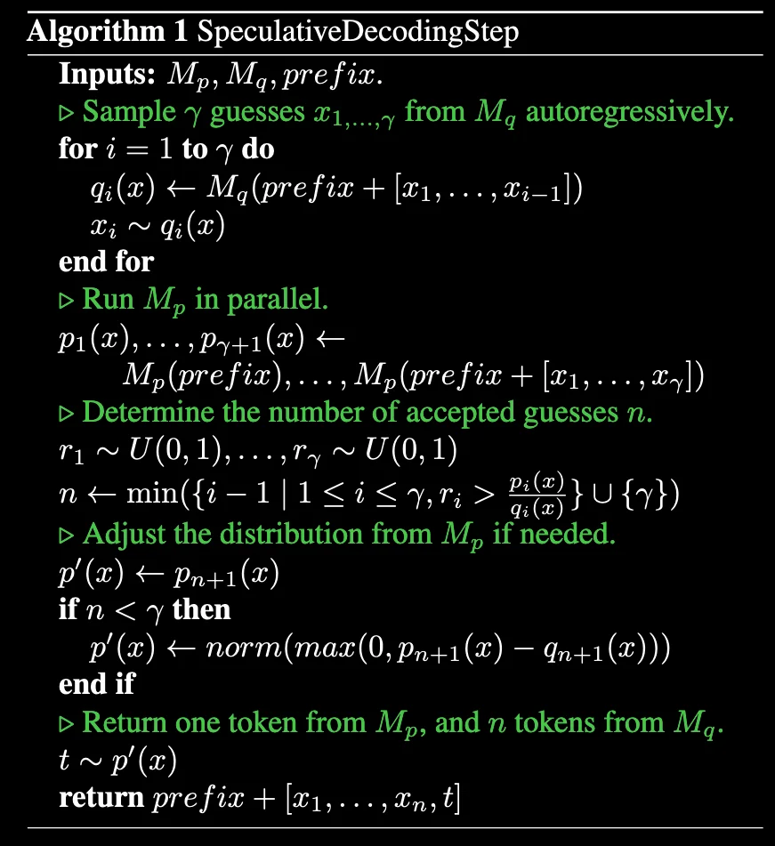
Algorithm 1 in detail

With these two concepts in mind, let’s go through algorithm 1 step by step. For your reference, below is the algorithm as specified in the paper.

Let’s say:

$M_p$ is a large and expensive autoregressive model
$M_q$ is a small and cheap approximation model
The current prefix (i.e. the tokens generated so far) is $y_{<t}$
The speculation length is $\gamma \geq 1$

The algorithm returns up to $\gamma$ new tokens (depending on how many is rejected. All of these evaluations of $M_p$ is done in one parallel batch.

Step 1: Speculative sampling via $M_q$

We first sample a sequence of $\gamma$ tokens from $M_q$ autoregressively.

Set $\tilde{\mathrm{x}} = [\;]$
For $i = 1$ to $\gamma$ :
1. Compute $q_i(\cdot) = M_q(y_{<t}, \tilde{x}_1, ..., \tilde{x}_{i-1})$
2. Sample a guess $\tilde{x}_i \sim q_i(\cdot)$
At the end, we should have $\tilde{\mathrm{x}} = (\tilde{x}_1, ..., \tilde{x}_\gamma)$

This costs $\gamma$ sequential forward passes for $M_q$ , but since $M_q$ is much cheaper than $M_p$ , we assume that this cost is “negligible” compared to one call of $M_p$ .

Step 2: Parallel evaluation by $M_p$

Next, we need to know the $p_i(\tilde{x}_i)$ for each speculative token $\tilde{x}_i$ to decide whether we accept this token or not.

In parallel, run $M_p$ on the following $(\gamma + 1)$ contexts:
$\begin{aligned}&\text{Context }1: \quad \mathbf{y}_{<t} \;\;\Longrightarrow\;\; p_{1}(\cdot),\\&\text{Context }2: \quad \mathbf{y}_{<t},\,\tilde{x}_{1} \;\;\Longrightarrow\;\; p_{2}(\cdot),\\&\quad\vdots\\&\text{Context }i: \quad \mathbf{y}_{<t},\,\tilde{x}_{1},\,\dots,\,\tilde{x}_{i-1} \;\;\Longrightarrow\;\; p_{i}(\cdot), \quad i = 1,\dots,\gamma,\\&\text{Context }(\gamma+1): \quad \mathbf{y}_{<t},\,\tilde{x}_{1},\,\dots,\,\tilde{x}_{\gamma} \;\;\Longrightarrow\;\; p_{\gamma+1}(\cdot).\end{aligned}$
Each of these $\gamma + 1$ context yield one distribution $p_i(\cdot)$ over $\mathcal{V}$
Note that we assume running $M_p$ in parallel does not incur any additional costs as compared to running $M_p$ once.

Step 3: Determine acceptance with rejection sampling

We now compare each $\tilde{x}_i$ with the true distribution $p_i$ . For $i = 1, …, \gamma$ :

Draw a uniform random number $r_i = \text{Uniform}(0,1)$
Compute the acceptance criterion:
$\rho_i = \frac{p_i(\tilde{x}_i)}{q_i(\tilde{x}_i)}$
Accept speculated token $\tilde{x}_i$ iff $r_i \leq \min(1, \rho_i)$ . $r_i$ effectively serves as the threshold

Let

n = \max \{k\in \{0, 1, ..., \gamma \}: \forall i \leq k \text{ were accepted}\}

Basically $n$ is exactly the number of accepted tokens before the first failure. For example:

If the first speculated token $\tilde{x}_1$ is rejected, then $n = 0$
If all $\gamma$ guesses are accepted, then $n = \gamma$

At this point, we know that $\tilde{x}_1, …, \tilde{x}_n$ are correct samples taken from the real distribution $p_1, …, p_n$ . Meanwhile, $\tilde{x}_{n+1}$ is rejected. We still need to determine how to produce a “true sample” for this token onwards.

Step 4: Fixing the distribution

In the case that there are some rejected tokens, we must re-draw the token from a rejection-corrected distribution $p’(x)$ . Let’s say the failure happens at token $n+1$ , as above.

The true distribution at that position is $p_{n+1}(\cdot)$
We already know that $q_{n+1}(\tilde{x}_{n+1}) > p_{n+1}(\tilde{x}_{n+1})$ , since that’s the precondition of the rejection (see step 3).
Define the “leftover” vector of $\mathcal{V}$
$L(z) = \max(0, p_{n+1}(z) - q_{n+1}(z)), \hspace{0.5cm} \forall z \in \mathcal{V}$
Normalize this leftover to get
$\begin{aligned} p'(z) &= \frac{L(z)}{ \sum_{y \in V} L(y)}\\ &=\frac{ \max\bigl(0,p_{n+1}(z) - q_{n+1}(z)\bigr)}{ 1 - \sum_{y \in V} \min\bigl(p_{n+1}(y),q_{n+1}(y)\bigr)} \end{aligned}$
Note the derivation of the denumerator can be done through careful observation.
Sample $y_{t+n} \sim p'(\cdot)$
Return the extended block $(\tilde{x}_1, …, \tilde{x}_n, y_{t+n})$

By construction, it is verified that we have recovered the same marginal for the $(n+1)$ -th token as if we had sampled it from $p_{n+1}$ . Therefore, speculative decoding reproduces the true next-token distirbution exactly while using cheap predictions from $M_q$ .

Designing $M_q$

A good $M_q$ candidate must be (1) much faster per token than $M_p$ to maximize speedups, (2) has sufficient overlap with $M_p$ for expected per-step token acceptance rate, $\alpha$ , to be reasonably high.

Options in the paper include:

n-Gram language model
- With bigram or trigram, inference is effectively just table lookups, practically with zero-cost
Tiny transformer models
- Take the same transformer model, but shrink the architecture to less layers with narrower hidden size
Heuristic copy models
- If the prefix appears in the context, guess the next token with high probability
- This is also a zero-cost approximation model
Non-autoregressive models
- Instead of running the approximation model sequentially, we can do only one forward pass.

Summary of key results

There are two main experiments conducted in the paper.

Empirical walltime improvement

Tested on T5 models, on machine translation and summarization tasks
Base model is T5-XXL with 11B parameters
As the size of approximation model increases, $\alpha$ increases
Shown that T5-small is the best approximation model yielding 2 to 3x speedups, regardless of the decoding strategy (greedy or sampling)
Other approximation models (T5-base and T5-large) also results in a ~1x to 2x speedups

Empirical $\alpha$ values

Tested on extra two models: GPT-like, with 97M parameters, and LaMDA with 137B parameters
The extra models are tested on dialog and text-generation tasks, while the T5 models are tested on the same tasks as above
Shown that tiny transformer models as the approximation model tend to perform best with $\alpha$ values between 0.5 to 0.9
Unigram and bigram models still stand to produce speedups. For example, in English to German translation, a bigram model results in 1.25x speedups to the original T5-XXL model
- However, the speedups from n-gram model is still lower than the speedups from tiny transformer models such as T5-small as the approximation model

My thoughts

I can clearly see why this paper is a landmark paper. It is very well-written, with strong theoretical foundation combined with clear empirical significance.

I can’t help but compare this method with knowledge distillation, as both are optimization methods leveraging a smaller model. It is quite interesting to note that knowledge distillation is more widely used (?), at least in my own experience with DeepSeek-R1 being distilled to LLaMA and Qwen models. Maybe there’s a way to combine both? What if we use distilled model as the approximation model? Would it improve the $\alpha$ by much?

Another method I am curious to see implemented in the speculative decoding context is the escalating framework from this paper. What if we start with n-gram models, and then slowly increase to larger models when the smaller models are unable to produce good $\alpha$ . Will this method results in worse performance than just using one approximation model? What would be the thereotical expected speedups using this escalation method? These are interesting avenues.

Other than that, great paper. Would love to implement the original vanilla speculative decoding for my work with Whisper soon.